Algebraic Coding Theory / Error Detection and Correction
First Lecture
History/Motivation
- Originated in the late 1940’s when Richard Hamming became frustrated with a mechanical relay model at Bell Telephone Laboratories that would lose all his information whenever a single error occurred.
- Today, possible transmission errors: human error, cross talk, lightning, thermal noise, impulse noise, and deterioration.
- Now used in compact disc players, fax machines, modems and bar code scanners.
- Gallian’s example: Consider sending a message to a Martian lander that interprets a 0 as a command to land, and a 1 as a command to orbit. Transmission error could cause the wrong message to be sent, so we must have a redundancy method.
Linear Codes
Formal Definition: An (n, k) linear code over a finite field F is a k-dimensional subspace of V of the vector space
Fn = F Å
F Å
F … Å
F
over F. The members of V are called the code words. A binary code would exist if n = 2.
Example 1: The set {0000, 0101, 1010, 1111} is a (4, 2) binary code.
Example 2: The set {0000000, 0010111, 0101011, 1001101, 1100110, 1011010, 0111100, 1110001} is a (7, 3) binary code
Example 3: A non-binary code: {0000, 0121, 0212, 1022, 1110, 1201, 2011, 2102, 2220} is a (4, 2) linear code over Z3 (a ternary code)
Hamming Codes
The Hamming (7, 4) code (1948)
|
Message
0000
0001
0010
0100
1000
1100
1010
1001 |
Code Word
0000000
0001011
0010111
0100101
1000110
1100011
1010001
1001101 |
Message
0110
1010
0011
1110
1101
1011
0111
1111 |
Code Word
0110010
0101110
0011100
1110100
1101000
1011010
0111001
1111111 |
This code, devised by Richard Hamming, is unique because it has the potential to correct an error should one occur.
For instance, if the message received were 0000011, we would decode on the assumption that one error occurred in the 4th spot, because the only expected code word that is within one number of the received word is 0001011. So we could deduce that the intended message was 0001.
Venn Diagram
We can illustrate how the Hamming (7, 4) code works by employing a Venn diagram. Essentially, this is three overlapping circles, which contain four shared areas. If we place our intended 4 digits inside each of these shared areas, the Hamming (7, 4) code works by placing the appropriate digits in the remaining spots in the independent portions of circles x A, B, and C so as to set the total sum of each circle equal to an even number. This summation trick is called a parity check.
If the message was sent to us, and we found that a circle contained an odd sum, we would know where to place the digit because of the interrelation between the circles. If only A summed to an odd number, we would know that the independent portion of A contained an error. If both A and B added up to an odd sum, we could deduce that the portion that is shared between A and B had an error during transmission.
The problem with both Hamming (7, 4) and the analogous Venn Diagram is that they are both faulty when more than one error occurs. To account for more than one error, codes with greater redundancy are needed.
Distance and Weight
Definition: Hamming distance – number of components in which two vectors differ.
Notation: d(u,v)
Definition: Hamming weight – minimum weight of any nonzero vector in the code.
Notation: wt(u)
Ex: u = 00011 v = 01001
u and v differ in 3 different locations, so d(u,v) = 3.
u has 2 non-zero digits, v has 3 non-zero digits, so wt(u) = 2, wt(v) = 2.
The reason we have these terms if because relationships exist between Hamming distance and Hamming weight. The most important Theorem follows:
Theorem of Hamming Distance and Hamming Weight (Theorem 1)
For any vectors u, v, and w:
d(u, v) = wt(u – v)
d(u, v) c
d(u, w) + d(w, v)
Proof (a.): Simply observe that both d(u, v) and wt(u – v) equal in the number of positions in which u and v differ
Proof (b): Let u and v differ in the ith position and u and w agree in the ith position, then w and v differ in the ith position.
Correcting Capability
If the Hamming weight of a linear code is at least 2t + 1:
- Then the code can correct any t or fewer errors.
- Alternatively, the same code can detect any 2t or fewer errors.
Proof (a):
- Suppose that a transmitted code word u is received as the vector v and that at most t errors have been made in transmission
- By definition of distance between u and v, we have d(u,v) c
t
- Let w be any code word other than u
- Then w – u is a nonzero code word.
- So 2t + 1 c
wt(w – u)
- By Theorem 1a above, wt(w – u) = d(w, u)
- By Theorem 1b above, d(w, u) c
d(w, v) + d(v, u)
- By step 2, we know that d(w, v) + d(v, u) c
d(w, v) + t
- Collectively, we’ve shown that 2t + 1 c
d(w, v) + t
- Simplified: t + 1 c
d(w, v)
Therefore, u is the closest vector to the code word we’ve received.
Proof (b):
- Suppose we receive the vector v when u is intended.
- Suppose at least one error, but no more than 2t errors, transmitted.
- Because only code words are transmitted, an error will be detected
whenever a received word is not a code word.
Algebraic Coding Theory / Error Detection and Correction
Second Lecture
What we’ve learned so far:
- Using redundancy increases the likelihood of a successful transmission.
- We can use algebraic coding to encode these redundancies in the most efficient manner possible.
- The type of algebraic code we are examining is called a linear code, expressed in the form (n,k)
- By analyzing concepts of Hamming distance and Hamming weight, we can determine the efficiency of these codes.
The Generating Matrix
Before, we showed that one potential generator of the Hamming (7, 4) code was:
G = [1 0 0 0 1 1 0
0 1 0 0 1 0 1
0 0 1 0 1 1 1
0 0 0 1 0 1 1 ]
The form of this generating matrix should look familiar. It carries a subspace V of Fk to a subspace of Fn in such a way that for any v in V, the vector vG will agree with v in the first k components and build in some redundancy in the last n – k components. This form is known as the standard generator matrix, and will always be of size k x n.
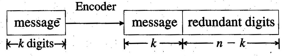
This form has the advantage that the original message constitutes the first k components of the transformed vectors. Any (n, k) code which uses a standard generator matrix is called a systematic code.
Example: Suppose we construct a generator for a (6, 3) linear code over Z2 for the set of messages: {000, 001, 010, 100, 110, 101, 011, 111}
G = [ 1 0 0 1 1 0
0 1 0 1 0 1
0 0 1 1 1 1 ]
The resulting code words that are generated by this systematic code are:
|
Message |
Encoder G |
Code Word |
|
000
001
010
100
110
101
011
111 |
è
è
è
è
è
è
è
è
è
|
000000
001111
010101
100110
110011
101001
011010
111100 |
Since we can see that the minimum weight of any nonzero code word is 3, this code will correct any single error or detect any double error.
Parity-Check Matrix Decoding
Now that we know how to encode our messages with redundancy measures, we’ll
need to have a way to decode these messages. This proves to be a bit more difficult, but we can at least show a simple method of decoding to compensate for at most one error. We can do this by creating a parity check matrix.
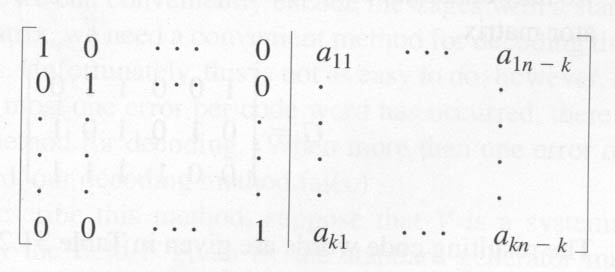
Consider the code which is given by the standard generator matrix G = [Ik | A], where Ik represents the k X k identity matrix and A is the k X (n – k) redundancy section of the generator. Therefore, we have an n X (n – k) matrix of the form:
How to Decode
|
Consider the generator matrix of the Hamming (7, 4) code:
G = [ 1 0 0 0 1 1 0
0 1 0 0 1 0 1
0 0 1 0 1 1 1
0 0 0 1 0 1 1 ]
|
The parity-check matrix of this generator is:
[1 1 0
1 0 1
1 1 1
H = 0 1 1
1 0 0
0 1 0
0 0 1 ]
|
We can decode a message by multiplying the received vector (v) with our parity-check matrix (H). If vH equals any single row of H, then we know the position of that row represents the position of an error in the transmitted message.
Example: If we receive a code message v = 0111101, then we know vH = 100.
Because 100 corresponds only to our parity-checking matrix’s fifth row, we can consider an error in the fifth digit of our received code message. Hence, we can determine the true code message should have been 0111001.
Orthogonality Relation
Let C be an (n, k) linear code over F with generator matrix G and parity-check matrix H. Then, for any vector v in Fn, we have vH = 0 (the zero vector) iff v belongs to C.
Parity-Check Matrix Decoding
Parity-check matrix decoding will correct any single error if and only if the rows of the parity-check matrix are nonzero and no one row is a scalar multiple of any other.
Coset Decoding
- Developed by David Slepian in 1956
- Conducted by constructing a standard array:
Example for a (6, 3) linear code C = {000000, 100110, 010101, 001011, 110011, 101101, 011110, 111000}
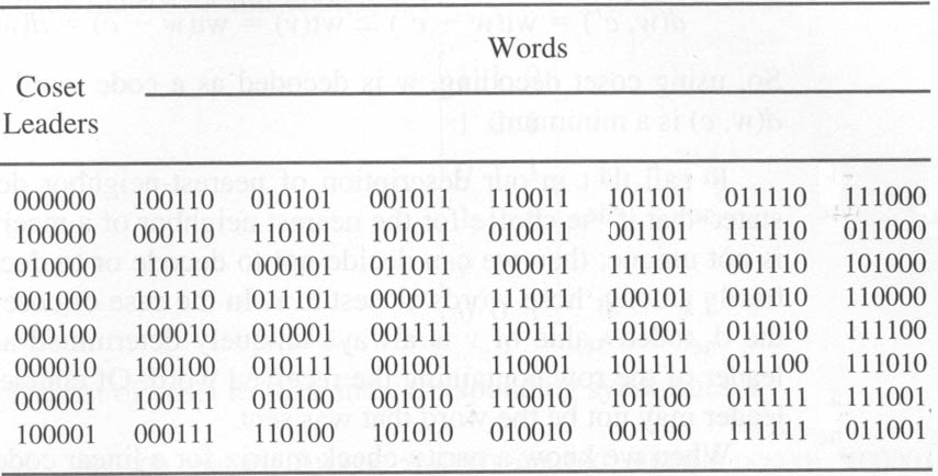
The first row of the standard array is just the elements of C as they would be received without any errors. Each of the rows beneath the first contain potential aberrations of a single error in the expected message at the top of the column. Notice that the first column is composed of all the coset leaders, and each has the minimum weight among the elements of its particular row. These represent the respective locations where an error has occurred.
Syndrome
Let C be an (n, k) linear code over F with a parity-check matrix H. Then, two vectors of Fn are in the same coset of C if and only if they have the same syndrome.
Medical terminology designates a "syndrome" as a collection of symptoms that typify a disorder. In coset decoding, the syndrome typifies an error pattern.
How to gather a syndrome:
- Calculate wH, the syndrome of w.
- Find the coset leader v so that wH = vH
- Assume that the vector sent was w – v.
Example: [ 1 1 0
1 0 1
G = 0 1 1
1 0 0
0 1 0
0 0 1 ]
H’s coset leaders and corresponding syndromes:
Coset leader 000000 1000000 010000 001000 000100
Syndromes 000 110 101 011 100
Coset leader 000010 0000001 100001
Syndromes 010 001 111
Let our received vector be v = 101001.
Compute vH = 100.
Since the syndrome 100 is related to the coset leader of 000100, we can assume v – 000100 = 101101 was the actual message sent.
Limitations of Analysis
- For the most part, we’ve only dabbled with Z2. More complicated number sets are used also.
- Standard generator matrices are vulnerable to damage loss in bursts
- More sophisticated coding theory makes greater use of group theory, ring theory and especially finite-field theory.
- One example is the ESA probe Giotto which visited Halley’s Comet in 1986. It utilized two error correcting codes. One checked for independently occurring errors, of which our standard generator matrices are an example of. The other code was a Reed-Solomon code which checked for bursts of errors, as many as thousands of consecutive errors. This is the same method that is now used on compact discs.
References:
Gallian, Joseph A. Contemporary Abstract Algebra. 4th ed. (Houghton Mifflin, 1998)
Lax, R. F. Modern Algebra and Discrete Structures (Louisiana State, 1991).
Thompson, Thomas M. The Carus Mathematical Monographs, Number Twenty-One: From Error-Correcting Codes Through Sphere Packings to Simple Groups. (MAA: 1983).